

When reading about earned value management and variance analysis, you most likely came across the cost variance (CV). Whether you’re controlling project costs or studying for the PMP test, knowing how to use the CV is critical to mastering project cost management.
The concept of cost variance is introduced in this article. It also includes definitions for the different CV types, as well as calculations and examples.

What Is Cost Variance?
The difference between a project’s earned value and actual expenses is measured by cost variance (CV). It is a component of the earned value management methodology (EVM) and a measure of the variance analysis technique. Some contend that this is also a component of the earned value analysis (EVA). However, this isn’t entirely accurate. EVA is a strategy for determining the input data (i.e., cost and value indicators) for cost and schedule variance calculations.
You may also like:
Free PMP Cheat Sheets and Formulas in 2021
How is Earned Value Calculated in Project Management?
Cost variations can be divided into three types:
There is point-in-time or period-by-period cost variance, cumulative cost variance, and variance at completion as a type of cumulative cost variance (VAC).
The definitions and differences of these types are discussed in the following sections.
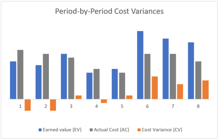
What Is Period-by-Period / Point-in-Time Cost Variance?
This is the most basic cost variation: The gap between actual cost and earned value within a certain period. As a result, it ignores any signs or variations from previous or future variances.
If you’re in month 4 of a project, for example, you’d calculate the point-in-time cost variance for that month solely using the actual cost (AC) and earned value (EV) of that month.
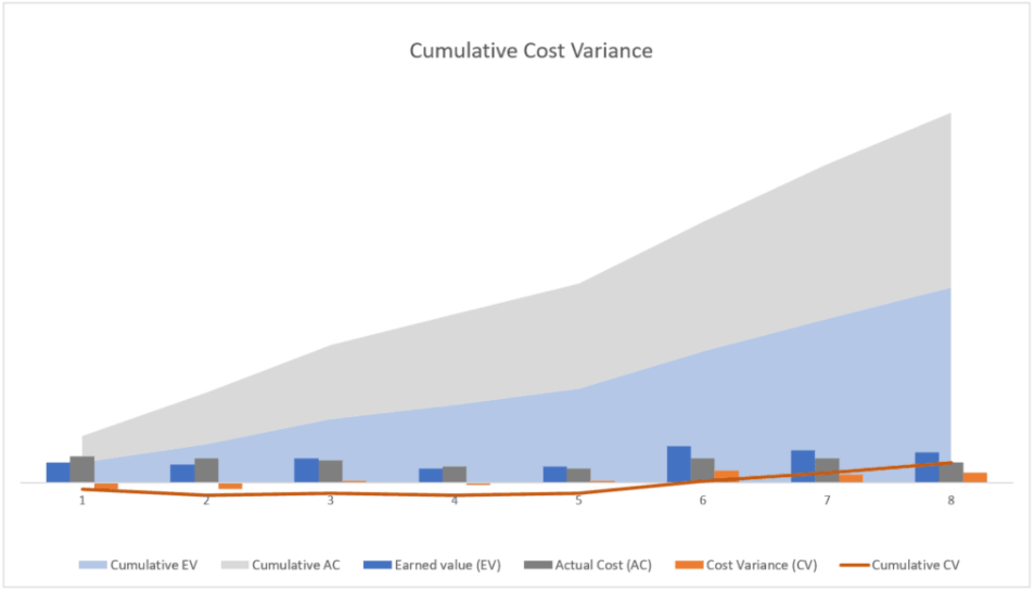
What Is Cumulative Cost Variance?
The cumulative CV measures the difference between the cumulative earned value and actual cost values across some periods, usually consecutively.
For example, suppose a project manager wants to determine the cumulative cost variance for the fourth month of a project. In that case, she must first calculate the cumulative earned value (EV) and cumulative actual cost (AC) for the fourth and previous months.
In other words, the difference between the sum of EV(1)+ EV(2)+EV(3)+EV(4) and the sum of AC(1)+AC(2)+AC(3)+AC(4) is the cumulative cost variance from the first to the fourth month.
What Is Variance at Completion (VAC)?
The cumulative cost variance at the end of the project is referred to as the variance at completion. The budget at completion (BAC) and the actual or expected cost at completion is the calculation parameters (EAC). The VAC is frequently used to measure forecasting approaches; More details can be found in this post regarding the estimate at completion (EAC).
How Is Cost Variance Calculated?
CV = EV – AC, where EV = Earned value and AC = Actual cost, is the basic formula for calculating cost variance.
Earned value (EV) refers to the portion of the budget allotted to work performed in a particular time or over several periods.
The actual cost (AC) is the cost or resources spent to complete the authorized task. It can refer to single or multiple periods (cumulative AC)
This formula must be modified to account for various types of cost variances. While the core formula – the difference between EV and AC – remains mostly the same, the following input parameters are substituted.
How Is the Period-by-Period Cost Variance Calculated?
The period-by-period or point-in-time cost variance is calculated using the fundamental formula and input parameters referring to a specific period:
CV (period) = EV (period) – AC (period)
The input parameters EV and AC refer to the work done and the cost incurred during the reference period. They don’t take into account numbers from any other period.
How Is the Cumulative Cost Variance Calculated?
Over several periods, the cumulative cost variance is calculated using the following formula:
CV (cumulative) = EV (cumulative) – AC (cumulative)

or CV (cumulative) = Sum of CV (all periods)
Where: CV (all periods) represents the sum of all point-in-time CVs for the periods under consideration.
The cumulative cost variance is frequently calculated from the start of a project to the most recent period. However, it can also refer to any other combination of periods; for example, a cumulative cost variance could be estimated for months 2 to 4, ignoring the first month and subsequent months.
Practice with SPOTO real test questions to assess your knowledge in Cost Variance (CV).
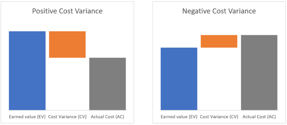
What Does the Calculated Cost Variance Values Mean?
A calculated cost variance’s value falls into one of the three value ranges below. Each one has a different meaning:
A negative cost variance (CV < 0) indicates a cost overrun, a favorable cost variation (CV > 0) shows that the earned value surpasses the actual cost, and a cost variance of zero shows that the budget was met, i.e., the actual cost and earned value are equal.
Contact us for more information on these indexes!
Cost Variance Calculation and Analysis Examples
The two examples below show how to calculate and use cost variances in a project. Because the cost-performance index (CPI) is typically employed in conjunction with these variances. It is worth noting that the input figures in the CPI article correspond to these samples.
You may also like: Free PMP® Sample Questions: Test Exam Cost Controlling & Earned Value Analysis
Example 1: A Straightforward Calculation of Cumulative and Point-in-Time Cost Variances
In the first example, the PMO’s earned value analysis yielded the following results:
| Month 1 | Month 2 | Cumulative numbers (month 2) | |
| Planned Value | 50 | 150 | 200 |
| Earned Value | 60 | 130 | 190 |
| Actual Cost | 50 | 170 | 220 |
Cost Variance Calculation
Using the formula AC = EV – AC, the project manager, computes two types of cost variances: cumulative and point-in-time cost variances.
| Month 1 | Month 2 | Cumulative numbers (month 2) | |
| Earned Value | 60 | 130 | 190 |
| Actual Cost | 50 | 170 | 220 |
| Cost Variance (CV) per period | 60 – 50 = 10 | -130 – 170 = -40 | – |
| Cost Variance, cumulative | – | – | 190 – 220 = -30 [or: 10 + (-40) = -30] |
The Calculated CV’s Interpretation
The total cost variance is unfavorable. This signifies that the total costs incurred so far surpass the earned value by a factor of 30.
The discrepancy between earned value and the actual cost is not insignificant in this scenario. Calculating the cost-performance index and the to-complete performance index might assist in analyzing this outcome and assessing its impact on the whole project.
When the cost variances are examined period by period, a more diversified picture emerges. While the cost variance was positive in the first month (i.e., the earned value surpassed the actual cost), it gradually became negative in the second month.
In this case, calculating point-in-time cost variations per period in addition to the cumulative cost variance may give the project manager an indication as to where to seek the core reasons for the cost overrun.
Example 2: A Case Study of a Project in Transition
In the second case, the PMO has established the following figures for the first three months of a project:
| Month 1 | Month 2 | Month 3 | Cumulative | |
| Planned Value | 100 | 130 | 200 | 430 |
| Earned Value | 60 | 120 | 220 | 400 |
| Actual Cost | 90 | 150 | 200 | 440 |
Cumulative and Period-by-Period CV Calculation
The cost variances are calculated by the project manager as follows:
Cumulative CV = 400 - 440 = -40
The negative cumulative cost variance, once again, indicates a cost overrun after the first three months of the project.
However, splitting it down into periods yields the following figures:
| Month 1 | Month 2 | Month 3 | Cumulative | |
| Cost Variance per period | -30 | -30 | 20 | -40 |
Cost Variances Interpretation
The first month’s cost variances shifted from a negative CV (m1) = -30 to a positive CV (m3) = +20 in the third month.
Such cost increases are relatively uncommon, given that projects and teams may need some “settling in” time before they can fully harness their performance potential. The change to a positive point-in-time cost variance in the third month, regardless of other internal and environmental factors, could indicate a good reversal in project performance.
The project manager may want to examine and facilitate the long-term viability of this beneficial development.
Conclusion
The cost variance is one of the core metrics of variance analysis, which is included in PMI’s Project Management Body of Knowledge as part of the earned value management approach (source: PMBOK®, 6th ed., ch. 7.4.2.2 Data Analysis, p. 261-264).
The CV itself reflects whether the cost of work accomplished during one or more project phases meets, exceeds, or falls short of the budgeted amount.
While this metric pertains to a project’s expense, the analogous indicator for the project’s timeline is the schedule variance (SV). The schedule performance index and the cost performance index are variations of these measures.
Last but not least, these metrics are part of the PMI methodology, a global standard for project management that is also covered in PMP and PMI-ACP certification tests. Practice with SPOTO real exam dumps and take SPOTO online training courses to strengthen your knowledge and earn your PMP or ACP certifications.
Comments